Lab 9: Hyperspectral remote sensing

Goals and Background:

In this lab hyperspectral data was introduced. The goal of the lab was to become familiar with various functions and procedures associated with this type of data. Hyperspectral data was atmospherically corrected using the FLAASH radiative transfer code method, hyperspectral signatures were plotted and compared to sample signatures, hyperspectral data was animated to show all bands, hyperspectral data was used in combination with various indecies to produce vegetation analysis data, and hyperspectral data was corrected for noise.

Methods:

Part 1 Section 1: Plotting hyperspectral signatures 

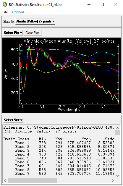
An JPL-calibrated AVIRIS image including 50 bands from 1.99 to 2.48 µm was brought into ENVI, and provided regions of interest of different minerals were opened after displaying the 183, 193, and 207 bands in RGB. Histograms for these ROIs were then opened and compared, paying special attention to features of the plots that could be used to identify one mineral from another. The samples used were of alunite, buddingtonite,calcite, and kaolinite. These ROI spectral samples were compared to library spectral samples that were brought in and plotted along with the ROI spectral samples.

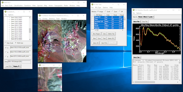Figure 1: Hyperspectral ROI spectral samples plotted

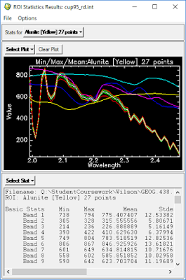Figure 2: Concurrent plots of ROI and library derived samples

Part 1 Section 2: Animating hyperspectral imagery

After loading the imagery into a new display window in grayscale by clicking on the file name instead of individual bands, the imagery was animated using the feature in the tools menu of the display window menu bar. In the resulting parameter window 20 bands for the animation were highlighted. Buttons changing the direction and speed of the animation were experimented with in order to assess and compare the bands that were animated.

Part 2: Atmospheric correction with FLAASH

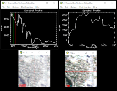
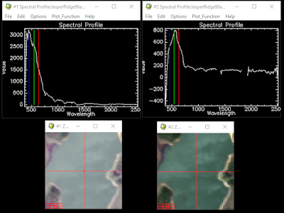
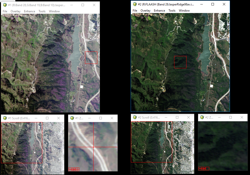
A separate AVIRIS image was opened in ENVI, and loaded in true color. By right clicking on the resultant image and selecting Z Profile the spectral profile of the image was opened. By right clicking on the image again and selecting Pixel Locator a specific area of the image was specified to be plotted. This area's plot showed the effects of oxygen, water, and CO2 absorption.

Figure 3: Jasper ridge hyperspectral imagery before (left) and after (right) FLAASH correction

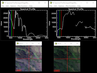
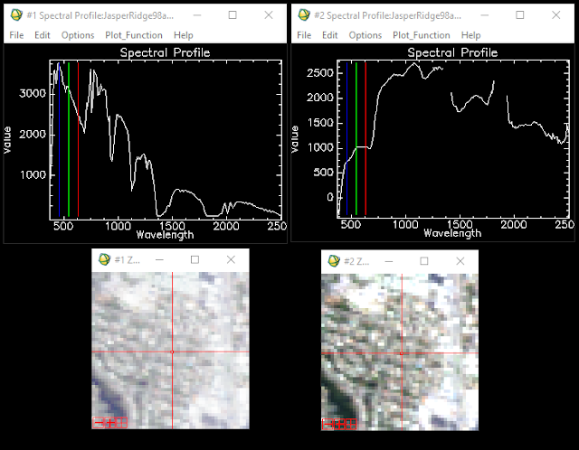
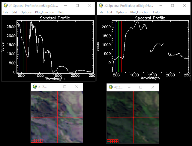
The FLAASH correction model tool was then opened from the Spectral folder of the ENVI menu bar. The image was input, the scale factors .txt file for integer to floating point conversion was input, and the other basic AVIRIS flight input parameters were entered. In the advanced settings window output template file generation was turned on: this is the only way for future inspection of FLAASH run instance parameters. The model was then run, and the corrected image brought into a new viewer for comparison. The spectral profile was opened and inspected: bad bands had been removed, and the effects of atmospheric absorption had been mitigated. The differences can be seen in Figures 4, 5, and 6. These show the specific changes for urban, vegetated, and water covered land.

Figure 4: Urban spectral change after FLAASH correction

Figure 5: Vegetation spectral change after FLAASH correction

Figure 6: Water spectral change after FLAASH correction

Part 3: Vegetation analysis

Another AVIRIS image was brought in and three bands (53, 29, and 19) were opened into a new RGB viewer. By using the Vegetation Index Calculator under the Spectral and then Vegetation Analysis menus all 25 indices were calculated with biophysical cross checking on. This feature compares the indices and corrects them. Multiple indices were then opened and inspected. The agricultural stress, fire fuel, and forest forest health tools were then opened and used to develop raster index images. These three tools are similar in operation. The parameter window for the fire fuel tool is shown in Figure 7.

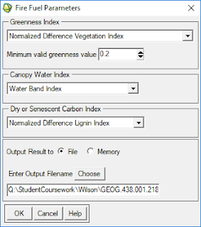Figure 7: Fire fuel tool parameters

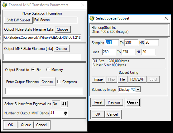
Part 4: Hyperspectral transformation

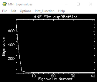
Using the minimum noise fraction transform, dimensionality and noise of an image were reduced. Noise statistics were estimated first, then the data was spectrally subsetted to 2.04 to 2.439, and finally parameters were entered. Noise stats were output, and the MNF process was run. The results were then brought into a viewer. Also output was a plot of Eigenvalues.

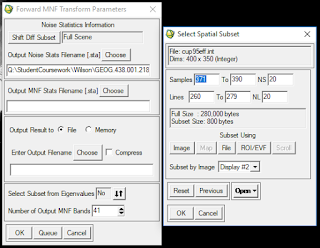Figure 8: MNF parameters

Results:

Part 1:

Part 1 resulted in an animation from which one could compare the reflectance across all bands of the hyperspectral image.

Part 2:

Part 2 resulted in a much darker image after the effects of atmospheric reflectance were removed. The before and after of this atmospheric correction process are shown in Figure 9. Before and after images for three separate areas, urban, vegetation, and water, are shown in Figures 10, 11, and 12 respectively.

Figure 9: Before and after atmospheric correction

Figure 10: Urban spectral change after FLAASH correction

Figure 11: Vegetation spectral change after FLAASH correction

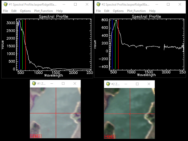Figure 12: Water spectral change after FLAASH correction

Part 3:

The results of the vegetation analysis procedures were many different index images, and then images from the three tools that were run. Theses are shown below in Figures 13, 14, and 15.

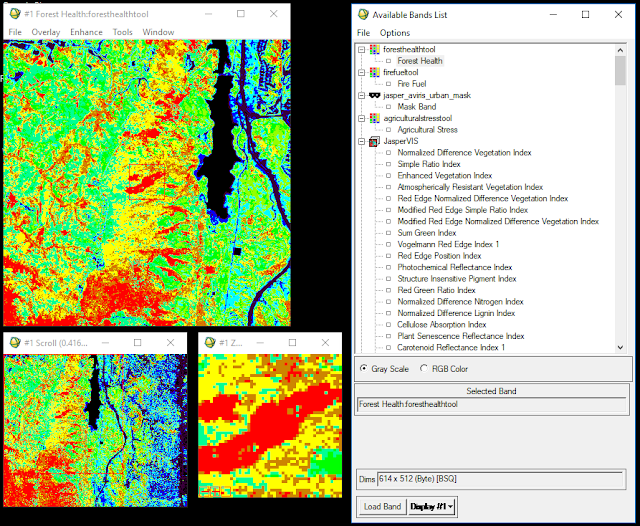Figure 13: Forest health tool results

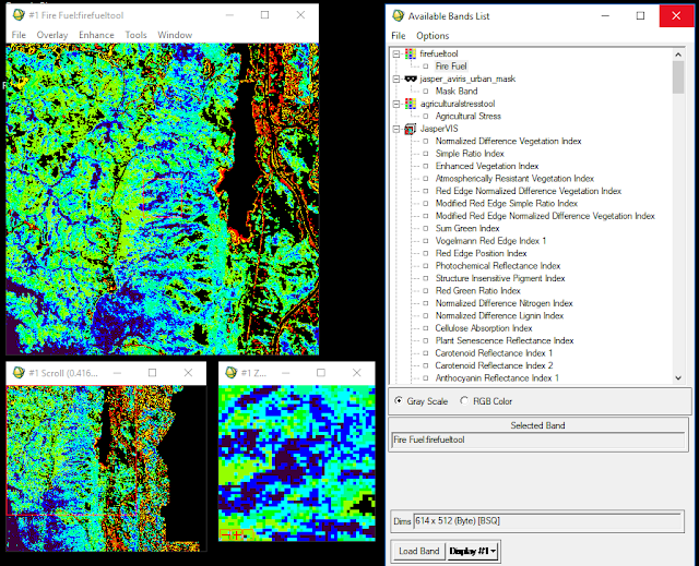Figure 14: Fire fuel tool results

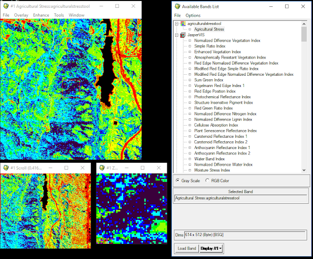Figure 15: Agricultural stress tool results

Part 4:

Part 4 resulted in an image with reduced noise and dimentionality and also a plot of eigenvalues. This plot showed the value nearing 1 at band 25, indicating near total noise.

Figure 16: Eigenvalue plot

Sources:

Instruction from Dr. Cyril Wilson. Data from Harris Geospatial.