Lab 10: Radar remote sensing

Goals and background:

The goal of this lab was to familiarize students with specific procedures associated with radar remote sensing images. The specific functions that were practiced were noise reduction (salt and pepper effect reduction) through speckle filtering, spectral and spatial enhancement, multi-sensor fusion, texture analysis, polarimetric processing, slant-range to ground-range conversion.

Methods:

Part 1 Section 1: Speckle suppression

25 m spatial resolution satellite (microwave) L-band remotely sensed images from the Shuttle Imaging Radar (SIR-A) experiment of the Lop Nor Lake in the Xinjiang Province of China were brought into ERDAS Imagine. The area includes a former lake bed with a basin area and also a cliff overlooking that basin. Figure 1 shows a regular oblique aerial image of the area found on Wikipedia.

Figure 1: Oblique aerial imagery of Lop Nor Lake

Speckle reduction was used to improve clarity of this image, this was found in the Utilities folder of the RadarToolbox in the Raster tab. The coefficient of variation is the first thing that has to be calculated for the image when using this tool. It's assumed that the noise follows a Rayleigh distribution. The coefficient of variation is the sqrt(variance)/mean. This can be calculated by simply running the tool with the box checked to find the coefficient. The coefficient is then output into the session log, and the tool is run again after inputting the coefficient as a parameter. The function can then be run in iterations to improve the effect. At each step a new coefficient of variation needs to be calculated. At each tool run instance the window size and the multiplier of the coefficient of variation are increased. In all three instances that were performed here, the Lee-Sigma filter was used. An alternative method that was suggested was to use the Lee filter for the first two passes, and the Local Region filer for the last pass of the algorithm.

Figure 2: The first pass of the speckle suppression filter

After running the filter's passes, the histograms were output for the files before and after the filter process. A side by side comparison of the images were also made. See results for these images and discussion.

Part 1 Section 2: Edge enhancement

In this section the Non-directional Edge tool was used that is located in the Spatial menu of the Resolution group of the Raster tab. The lake image was run through the filter, as well as the 3-pass despeckle image. The image that had only passed through the edge enhancement tool was then run through the despeckle tool for comparison on the results from the different orders of processing. These results can be seen in the results section. The parameters used for the Non-directional edge tool are shown below in Figure 3.

Figure 3: Non-directional Edge tool parameters

Part 1 Section 3: Image enhancement

In this section, a radar image of a glacier was brought into ERDAS Imagine, and was run through the Speckle Suppression filter first. The Gamma-MAP filter was used for this image. THe image was then run through the Wallis Adaptive Filter tool. The stretch to unsigned 8 bit option was used, as well as a window size of 3 and a multiplier of 3.00. The small multiplier was used due to the roughness of the image. The results were then viewed, and are shown below in the Results section.

Figure 4: Wallis Adaptive Filter tool parameters

Part 2 Section 1: Application of Sensor Merge

In this section a Landsat TM reflective bands image, and a radar active sensor image are combined using the IHS Intensity method and stretching to unsigned 8 bit, and bands 1, 2, and 3, assigned to R, G, and B. 

Figure 5: Sensor Merge tool

Part 2 Section 2: Application of Texture Analysis

In this section, the Texture Analysis tool was applied to a radar image of agricultural land in Flevoland, Holland taken by the ERS-1 satellite in C-band with a 20 meter spatial resolution. The tool was found under the Utilities folder of the RadarToolbox in the Raster tab. The moving window was set to 5, and the Skewness operator was chosen.

Part 2 Section 3: Brightness Adjustment

Brightness adjustment simply adjusts each line of the image to have the same average. This is processed by using the Brightness Adjustment tool in the Utilities folder of the RadarToolbox in the Raster tab. The column option was chosen for the data that was used after reading its header file, and then the image was processed.

Part 3 Section 1: Synthesizing SIR-C Images

In this section L-band single look complex (SLC) SIR-C images of a Death Valley section of alluvial fans were synthesized for specific polarizations from the compressed matrix output file provided. The data used had a range resolution of 13 m and an azimuth size of 5 m. Multilooking had already been performed to make 13 m square pixels.

After selecting the Synthesize SIR-C Data option from the Radar > Polarimetric Tools menus, the file was brought in and the tool was run. All four normal transmit/receive polarization combinations were selected by default (HH, VV, HV, and TP), and the byte data output option was selected. Then, other polarization combinations were created by running the tool again but specifying -45 in both the Transmit Ellip and Receive Ellip fields and 135 in the Transmit Orien and Receive Orien fields, and then 0 in both the Transmit Ellip and Receive Ellip fields and 30 in the Transmit Orien and Receive Orien fields. This produced first a right-hand circular polarization, then a linear polarization image. The image this time was output in dB. The images were then displayed and the interactive stretching enhancement was turned on for the images. Linear, square root, and Gaussian stretching techniques were used. An RGB image was also displayed using the HH band in red, VV in green, and HV in blue.

Figure 6: Standard polarization combinations synthesis

Figure 7: Other polarization cominations synthesis

Results:

Part 1 Section 1: Speckle suppression

The histograms below show the lake bed after two passes (left) and the lake bed unfiltered (right). The histogram's shape not only became bi-modal, but the spikes from the image were also reduced in the despeckle process.

Figure 8: Histogram change after two passes of the speckle suppression filter

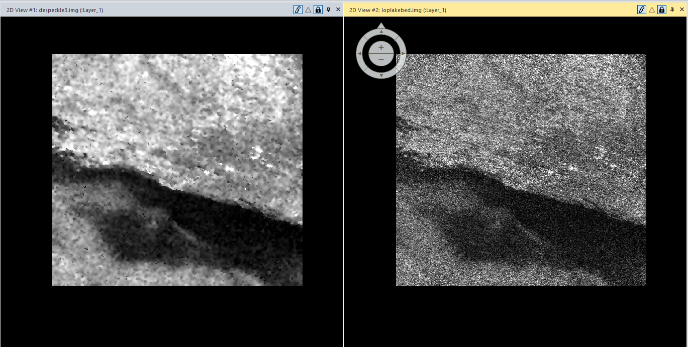
Below in the side by side comparison of the despeckle process (left image is processed) it is apparent that the despeckle process removed a lot of noise, but also made the image less clear (lower resolution). In using these images for analysis or in presenting these images it seems that the best way of analysis is to show both (or more) images. In some versions of the image some aspects of the image are clearer than in other versions of the image.

Figure 9: Results of the despeckle process (left is processed, right is original image)

Part 1 Section 2: Edge enhancement

Below are the results of the two different orders of edge enhancement and speckle reduction processing. On the right is the speckle reduction first and edge enhancement second file, and on the left is the edge enhancement and then speckle reduction result file. Depth is much more apparent in edges.img than in the image where the despeckle function was run second to the edge, however the consistency of the shading makes the edge first, despeckle second image easier to interpret in terms of surfaces. The edges.img image has small curvy lines that are distracting from the features that they make up. The edge of the cliff is very easy to find in the edges.img file though.

Figure 10: Edge enhancement and despeckle processing order comparison

Part 1 Section 3: Image enhancement

The results of the image enhancement were to lower the resolution and to stretch the contrast. The processed image looks smoother, although I think that less detail can be seen. The speckle was effectively mitigated, however, and the processed image has less range in contrast as well, but not by a lot, making the noise reduction of the process apparent.

Figure 11: Image enhancement (Wallis Adaptive Filter) result and original data

Part 2 Section 1: Application of Sensor Merge

The results below show the interesting to interpret results of the Sensor Merge tool. The resulting image from the TM and the radar images takes on the depth values of the radar image and also the color of the TM image. The result is an interesting combination, because since the clouds are tinted red, much of the green land cover is tinted red. Also it is hard to interpret because there are two different kinds of data contributing to the color and brightness values of the resultant image. The original TM image has a lot of clouds obscuring the picture of the ground, and the radar image shows depth, but little other context as to the date the image was taken or other elements of the nature of the image is given. The resulting image seems to take on weird colors compared to the TM image in places and this may be due to the influence of the radar image. It may also have to do with displaying the image in 1, 2, 3 form instead of 3, 2, 1 real color mixing.

The image below shows the mixed image on the left, the radar image on the top right, and the TM image on the bottom right. This seems to be another case where the analyst needs to have all layers open to interpret and use the results of the merged image.

Figure 12: Sensor Merge results and original radar and TM images

Part 2 Section 2: Application of Texture Analysis

The resulting image shows the outlines of the areas of similar value, showing the boxy texture of the land (below, right). The original image simply shows the values of the image (left), which make it easier to interpret what type of land cover is there, but not what the general texture of that land is.

Figure 12: Texture analysis results and original image

Part 2 Section 3: Brightness Adjustment

I tried two passes but the second pass doesn’t seem to have changed the first pass. The first pass seems to have brightened bright areas and darkened dark areas. Looking at the histogram, it seems that the max value hasn’t changed much, but the min has, and it’s negative. This means that many more pixels will be displayed as 0 than before, as negative values don’t exist. In the image directly below, the adjusted image is on the right, and the original is on the left.

Figure 13: Brightness adjustment results and original image

Part 3 Section 1: Synthesizing SIR-C Images

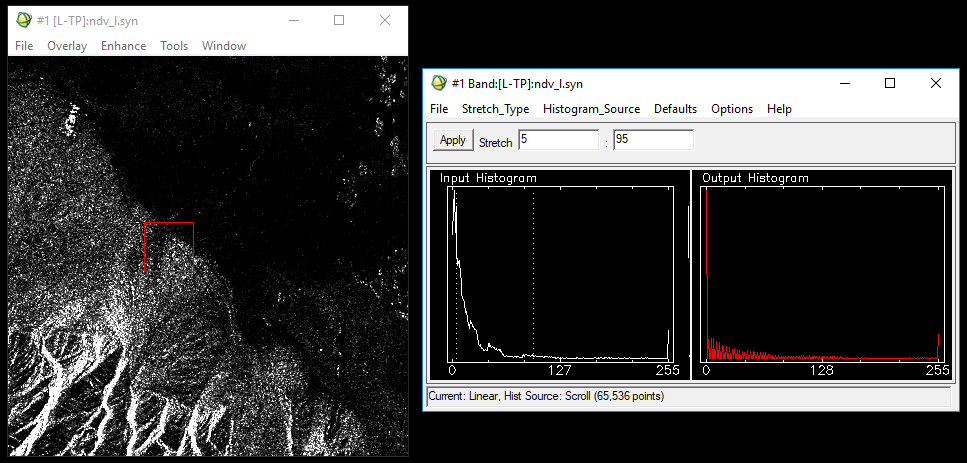
Below are the three stretching techniques, all stretching using the same start and end values. The linear stretch kept pixels the darkest, while the square root stretch was the next brightest, and the brightest was the Gaussian method. When looking at the histograms it became clear why: the Gaussian distribution stretch brought pixels from the values between 5 and 95 to higher values than the other methods had.

Figure 14: Linear stretch result

Figure 15: Gaussian stretch result

Figure 16: Square root stretch result

This next image is the color image generated with the HH polarization combination band in red, VV in green, and HV in blue. The image was Gaussian stretched from 0 to 130 to brighten the image slightly. The histogram is useful for this image in observing differences between the three polarization combinations in a single area.

Figure 17: Multiple polarization combination color image with applied Gaussian stretch

Sources:

Data from Erdas Imagine (2016) and ENVI (2015). Instruction from Dr. Cyril Wilson.