Lab 7: Object-based classification
Goals and Background:
The objective of this lab was to become familiarized with object-based land use/land cover (LULC) classification performed in Trimble eCognition. This process is made up of a few different processes: first segmentation of images into objects (clusters of pixels grouped based on spatial and spectral homogeneity vectorized), then training and setup of random forest and then support vector machine classifiers, and finally refining of the classification output from the classifiers.
Methods:
Part 1: Creating the eCognition project
A new project was created in eCognition using Landsat 7 ETM+ imagery supplied from June 9, 2000. The data brought in included the 6 bands from the sensor, however which bands these were was unspecified. The resolution of the imagery was set at 30 meters as this was the spatial resolution of all of the layers, and a global value of zero was set for cases of no data.
The layer mixing button was now clicked in the top bezel , and the layers were mixed with the resulting screen to show a 4, 3, 2 false infrared image for ease in interpretation (Figure 1).
Part 2 Section 1: Creating image objects
New events were now created in the process tree. A parent event was created called "Generate Objects" under which a child process to perform the segmentation process was created. The segmentation process was edited to be as shown in Figure 2. The shape and compactness weight parameters were set to 0.3 and 0.5 respectively, the level was set to 1 (only first level classification was performed), and the scale parameter was set to 9. Smoothness describes the similarity between the image object borders and a perfect square. Compactness describes the closeness of pixels clustered in an object by comparing it to a circle.
The segmentation was now executed.
Part 2 Section 2: Training Sample Selection
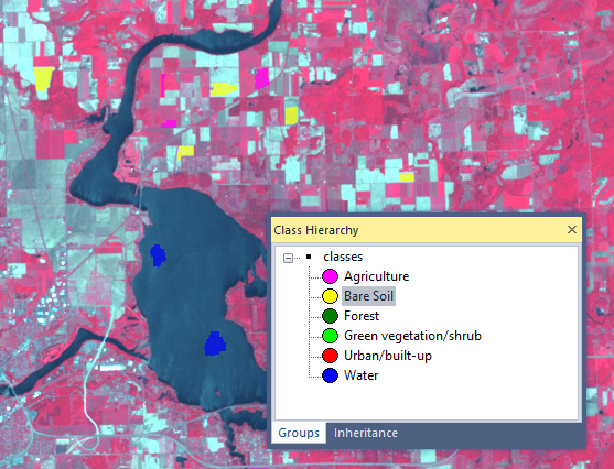
Using unique colors for every class, classes were created in the Class Hierarchy window. Much like a pixel-based supervised classification, samples now had to be created for training the classifier. The samples were collected by selecting the option under the Classification menu. Classes used can be seen in Figure 3, and a selection of samples is shown in Figure 4.
Part 3 Section 1 and 2: Apply the Random Forest classifier using the sample objects
Parts 1-3: Random Forest classifier
The Random Forest classifier worked well (much better than any pixel-based classifier) at classifying the image after experimentation with collecting different samples. Though there was a lot of bare soil land cover that was classified as urban land, this could easily be fixed with more tinkering with samples or a post machine learning classification expert system/decision tree classification. All other LULC classes were fairly accurately classified.
Part 4: Support Vector Machine classifier
The SVM classifier created an almost identical image to the Random Forest classified image. The same samples were used in the two classifications for comparison between the two classifiers and also the same characteristics of the objects were used (all of the bands means, brightness, max diff., GLCM dissimilarity, and GLCM mean). Because these were all the same, the difference between the two classifiers that may be there should have become apparent, but it seems that at least with the characteristics of the samples and objects to be classified that were used here, there is no difference. If less training data and less skillfully chosen training statistics and properties were used a difference may be able to be shown, however this is only speculation.
Part 5: Random Forest classifier used with UAS data
The UAS imagery's classification was successful besides the vehicle class. This is because all of the vehicles has widely different colors and reflections of bright light in some places, making consistent samples difficult to collect. If I had been in charge of creating the scheme for this classification, I would not have included cars.
Sources:
UAS imagery was sourced from the UW - Eau Claire Geography Department Faculty. Landsat imagery is from the Earth Resources Observation and Science Center of the US Geological Survey.
The objective of this lab was to become familiarized with object-based land use/land cover (LULC) classification performed in Trimble eCognition. This process is made up of a few different processes: first segmentation of images into objects (clusters of pixels grouped based on spatial and spectral homogeneity vectorized), then training and setup of random forest and then support vector machine classifiers, and finally refining of the classification output from the classifiers.
Methods:
Part 1: Creating the eCognition project
A new project was created in eCognition using Landsat 7 ETM+ imagery supplied from June 9, 2000. The data brought in included the 6 bands from the sensor, however which bands these were was unspecified. The resolution of the imagery was set at 30 meters as this was the spatial resolution of all of the layers, and a global value of zero was set for cases of no data.
The layer mixing button was now clicked in the top bezel
 , and the layers were mixed with the resulting screen to show a 4, 3, 2 false infrared image for ease in interpretation (Figure 1).
 |
| Figure 1: Layer mixing |
New events were now created in the process tree. A parent event was created called "Generate Objects" under which a child process to perform the segmentation process was created. The segmentation process was edited to be as shown in Figure 2. The shape and compactness weight parameters were set to 0.3 and 0.5 respectively, the level was set to 1 (only first level classification was performed), and the scale parameter was set to 9. Smoothness describes the similarity between the image object borders and a perfect square. Compactness describes the closeness of pixels clustered in an object by comparing it to a circle.
The segmentation was now executed.
 |
| Figure 2: Segmentation parameters |
Using unique colors for every class, classes were created in the Class Hierarchy window. Much like a pixel-based supervised classification, samples now had to be created for training the classifier. The samples were collected by selecting the option under the Classification menu. Classes used can be seen in Figure 3, and a selection of samples is shown in Figure 4.
 |
| Figure 3: Classes for SVM and Random Forest classification |
 |
| Figure 4: A selection of training samples |
Another parent event was created "RF Classification". Under this event are two child events: "Train RF Classifier", and "Apply RF Classifier". Under the "Train RF Classifier" event is an event that trains the classifier after the user defines parameters. Under the "Apply RF Classifier" event is another event that applies the classifier. The parameters for classifier training are shown in Figure 5, and the parameters for the application of the classifier are the same besides that the Operation chosen is Apply.
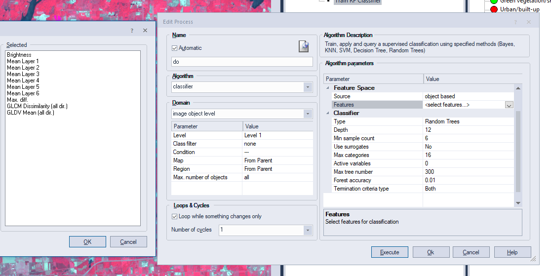 |
| Figure 5: Random Forest classifier training parameters |
The spectral characteristics of the objects chosen for the classifier to work with were brightness, means of all of the layers, max difference, GLCM dissimilaity (all dir.), and GLCM Mean (all dir.). These had been tested and shown to work the best with the data and type of classification we were using. The other parameters chosen were a depth of 12, a min sample count of 6, and a max tree number of 300.
The entire process tree is shown in Figure 6. This process tree's structure was used in the subsequent classification processes in this lab regardless of classifier.
 |
| Figure 6: Classification process tree |
Part 3 Section 3: Refining classification by editing signatures
By selecting the class filter and selecting the classes that needed to be edited in the apply classifier event, and using the manual editing toolbar, the classes that needed to be changed for a better classification were edited. The classifier was then executed again after the necessary edits were made.
Part 3 Section 4: Export classified image
By selecting Export Results under the Export menu, the results of the classification could be exported. The results were exported as a raster image which was then brought to ArcMap to make a figure.
Part 4: Support Vector Machine (SVM) classifier
The same process was used to perform the SVM classification of the same Landsat 7 ETM+ image, but with SVM chosen as an event parameter several times. The same spectral characteristics of the objects were used for training, and all other default parameters were chosen.
Part 5: Object-based classification of UAS imagery
Object-based Random Forest classification of an image that was collected using a UAS was now performed. All of the same parameters from the previous Random Forest classification were able to be used successfully with this image besides the scale parameter in the earlier stage of segmentation of the image. Instead of a scale parameter of 9, this high resolution imagery's scale parameter was set to around 190. Classes used with this large scale imagery (although having a small extent of ground coverage) were buildings, trees, roads, vehicles, and lawns.
Results:
Parts 1-3: Random Forest classifier
The Random Forest classifier worked well (much better than any pixel-based classifier) at classifying the image after experimentation with collecting different samples. Though there was a lot of bare soil land cover that was classified as urban land, this could easily be fixed with more tinkering with samples or a post machine learning classification expert system/decision tree classification. All other LULC classes were fairly accurately classified.
 |
| Figure 7: Random Forest classification results |
Part 4: Support Vector Machine classifier
The SVM classifier created an almost identical image to the Random Forest classified image. The same samples were used in the two classifications for comparison between the two classifiers and also the same characteristics of the objects were used (all of the bands means, brightness, max diff., GLCM dissimilarity, and GLCM mean). Because these were all the same, the difference between the two classifiers that may be there should have become apparent, but it seems that at least with the characteristics of the samples and objects to be classified that were used here, there is no difference. If less training data and less skillfully chosen training statistics and properties were used a difference may be able to be shown, however this is only speculation.
 |
| Figure 8: SVM classification results |
Part 5: Random Forest classifier used with UAS data
The UAS imagery's classification was successful besides the vehicle class. This is because all of the vehicles has widely different colors and reflections of bright light in some places, making consistent samples difficult to collect. If I had been in charge of creating the scheme for this classification, I would not have included cars.
 |
| Figure 9: Random Forest classifier preformed with UAS imagery |
UAS imagery was sourced from the UW - Eau Claire Geography Department Faculty. Landsat imagery is from the Earth Resources Observation and Science Center of the US Geological Survey.


Comments
Post a Comment